High-Order Butterworth Filters, Time and Frequency Analysis
Continuous-Time Transfer Function
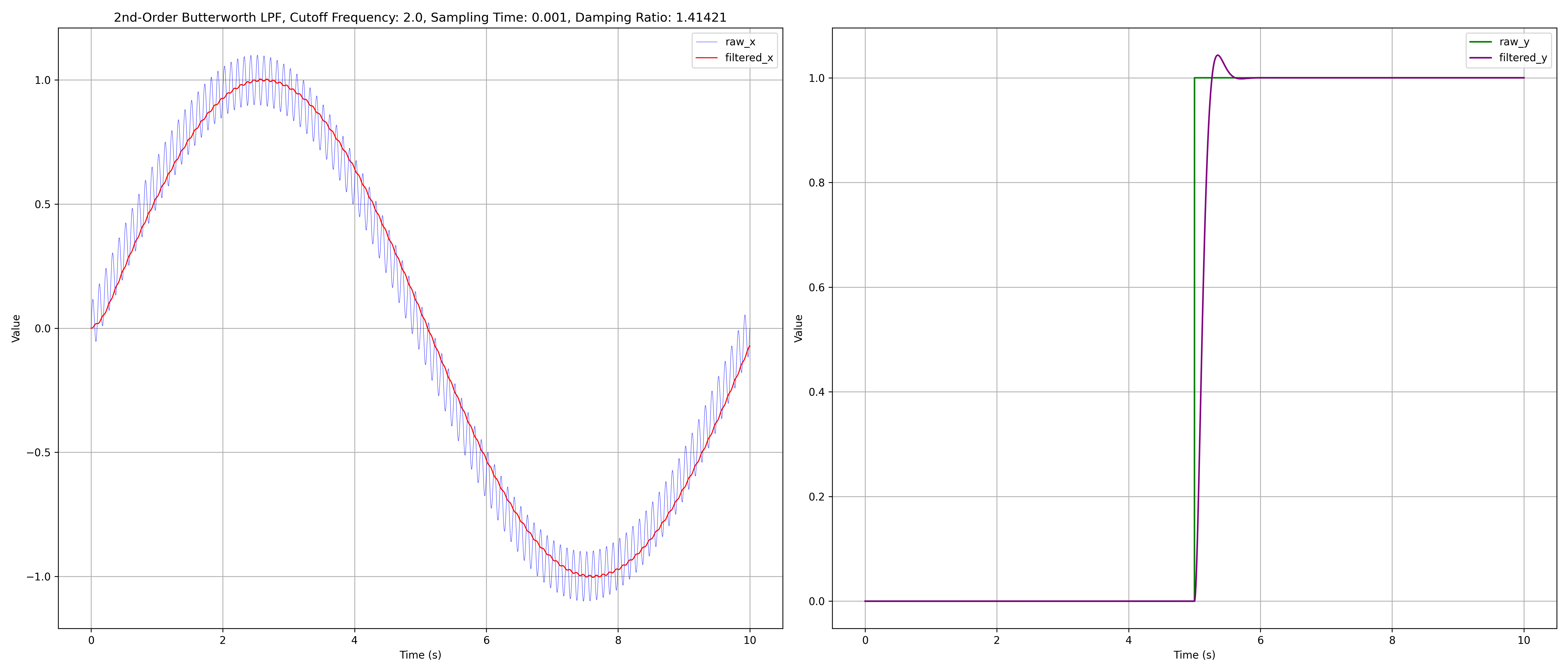
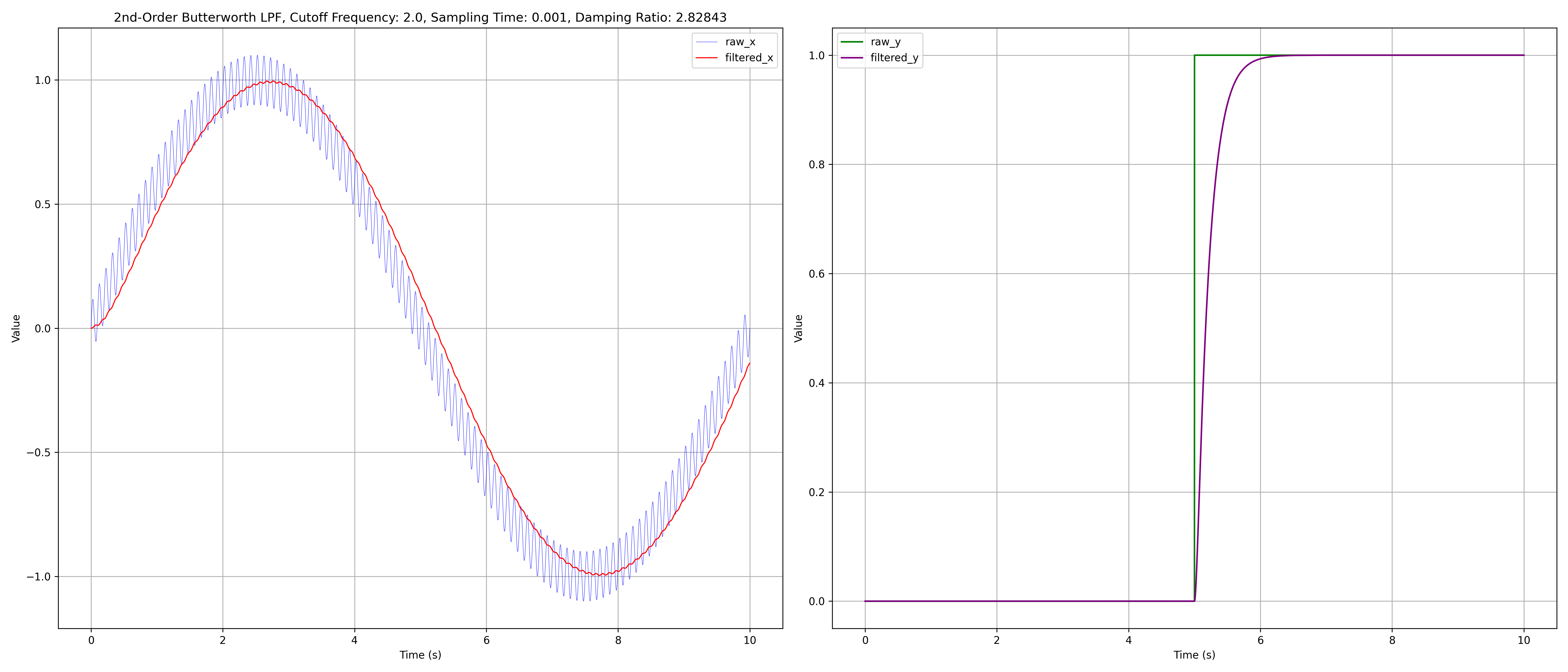
For a second-order butterworth low-pass filter, it is given by $$ H(s) = \frac{\omega_c^2}{s^2 + \xi \omega_c s + \omega_c^2} $$ where
- $ \xi = \sqrt{2} $ is the underdamped damping ratio,
- $ \omega_c $ is the cutoff frequency in rad/s.
Discrete-Time Transfer Function and Difference Equation
Software implementation of the above filter requires its difference equation, steps to derive that are as follows.
Compute pre-warp cutoff frequency to compensate for the distortion caused by later taking the bilinear transformation $$ \omega_c' = \frac{2}{T} \tan \left( \frac{\omega_c T}{2} \right) $$ $$ T = \frac{1}{f_s} $$ rectify continuous time transfer function $$ H(s) = \frac{\omega_c'^2}{s^2 + \sqrt{2} \omega_c' s + \omega_c'^2} $$ take bilinear transformation $$ s = \frac{2}{T} \frac{1 - z^{-1}}{1 + z^{-1}} $$ get the discrete time transfer function $$ H(z) = \frac{b_0 + b_1 z^{-1} + b_2 z^{-2}}{1 + a_1 z^{-1} + a_2 z^{-2}} $$ convert to difference function $$ y[n] = b_0 x[n] + b_1 x[n-1] + b_2 x[n-2] - a_1 y[n-1] - a_2 y[n-2] $$ with coefficients $$ b_0 = \frac{1}{1 + \sqrt{2} K + K^2} $$ $$ b_1 = 2b_0 $$ $$ b_2 = b_0 $$ $$ a_1 = 2(1 - K^2) b_0 $$ $$ a_2 = (1 - \sqrt{2} K + K^2) b_0 $$ $$ K = 1/ \tan\left(\frac{\pi f_c}{f_s}\right) $$
C++ implementation of a 2nd-order butterworth low-pass filter.
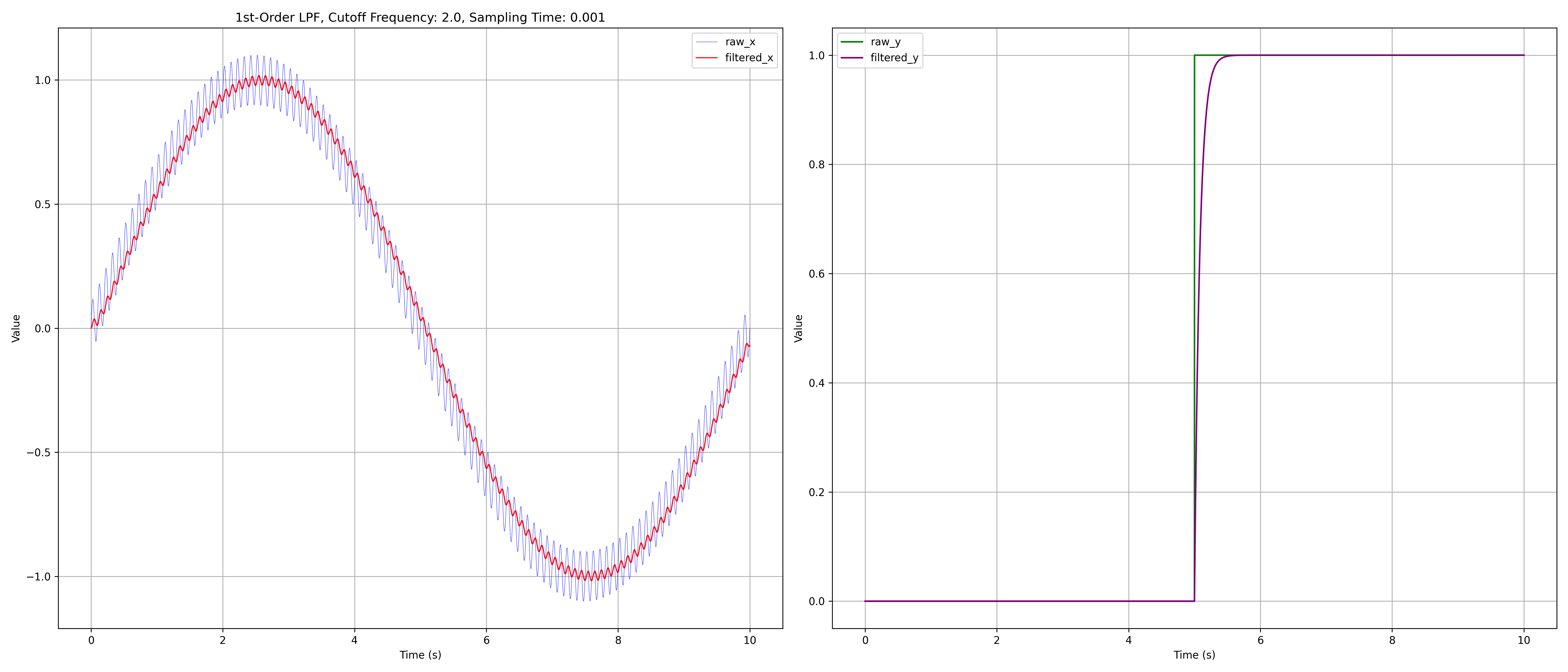
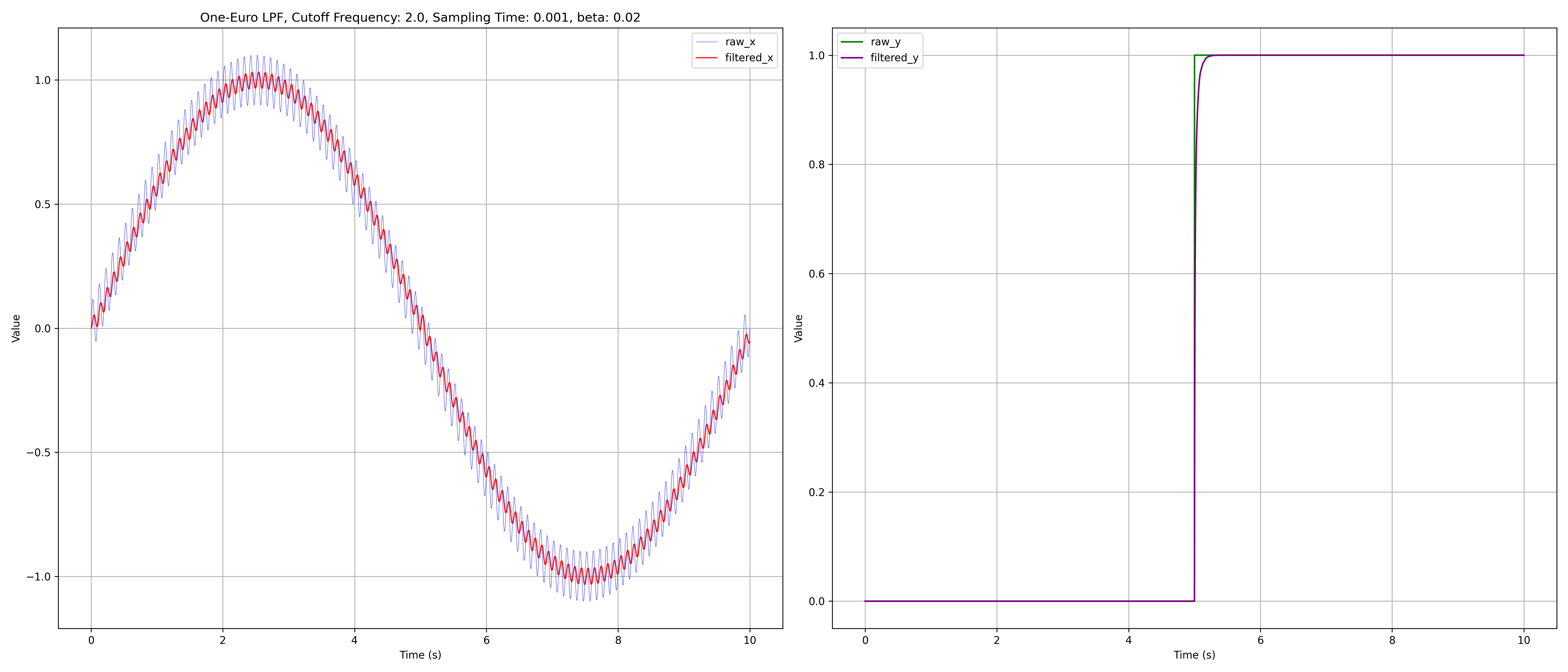
Comparison between the above 2nd-order butterworth low-pass filter and First-Order Low-Pass Filters in Rn and SE(3) with similar parameters.
C++ implementation of a 3rd-order butterworth low-pass filter is similar.
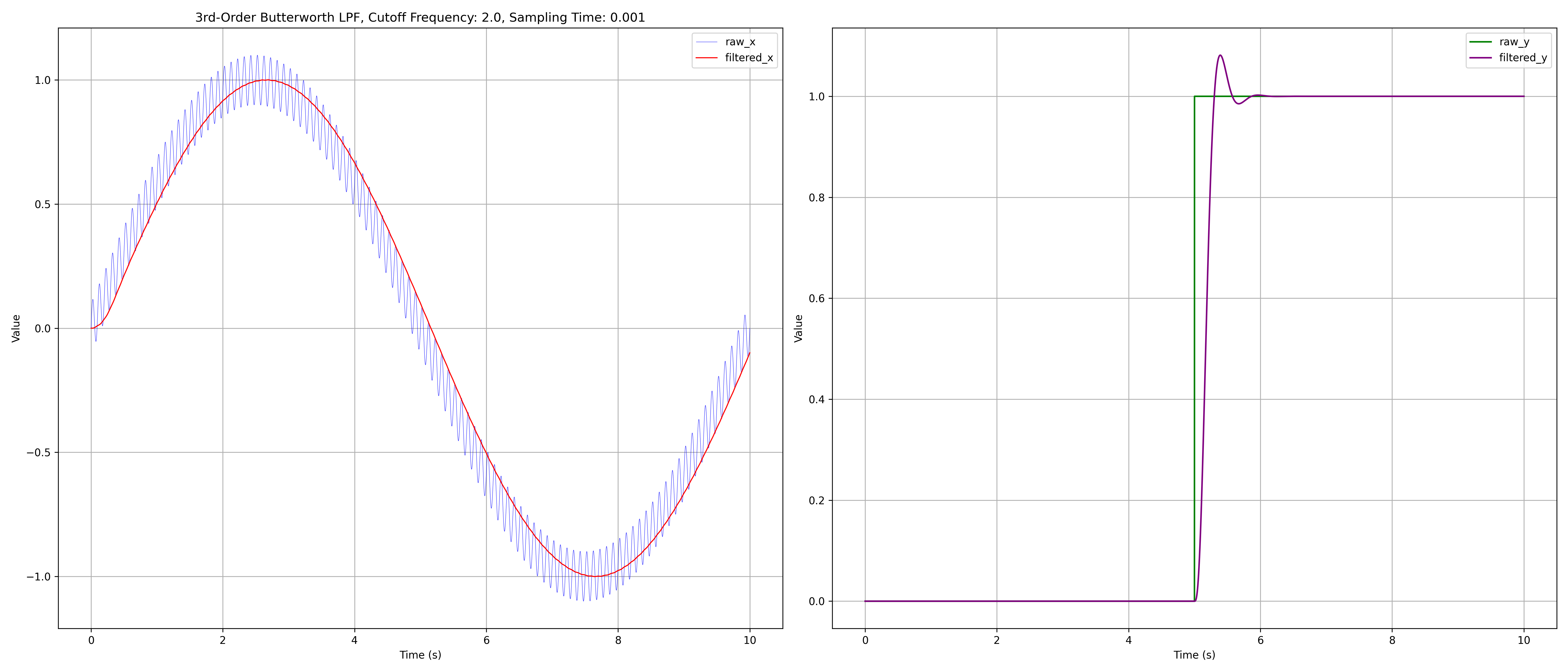
Comparison between standard 2nd-order and 3rd-order butterworth low-pass filters with same parameters.
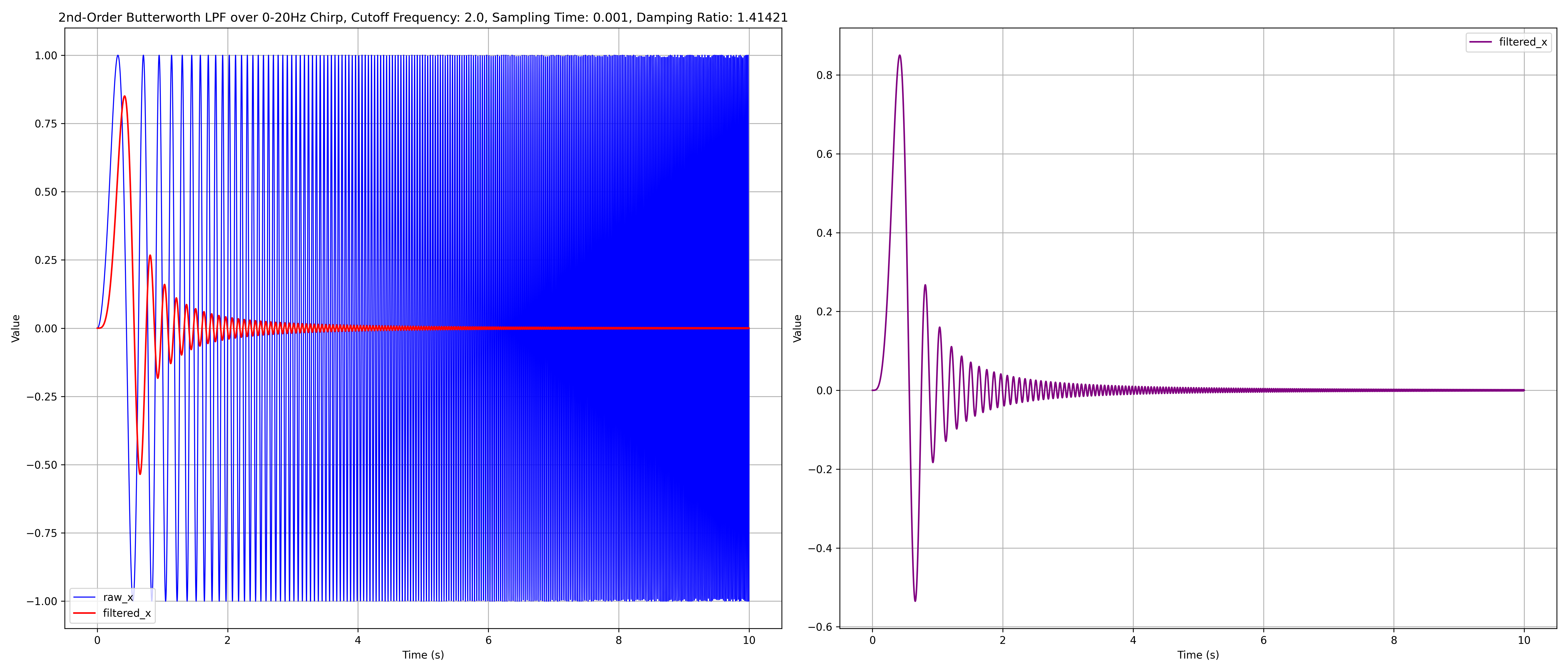
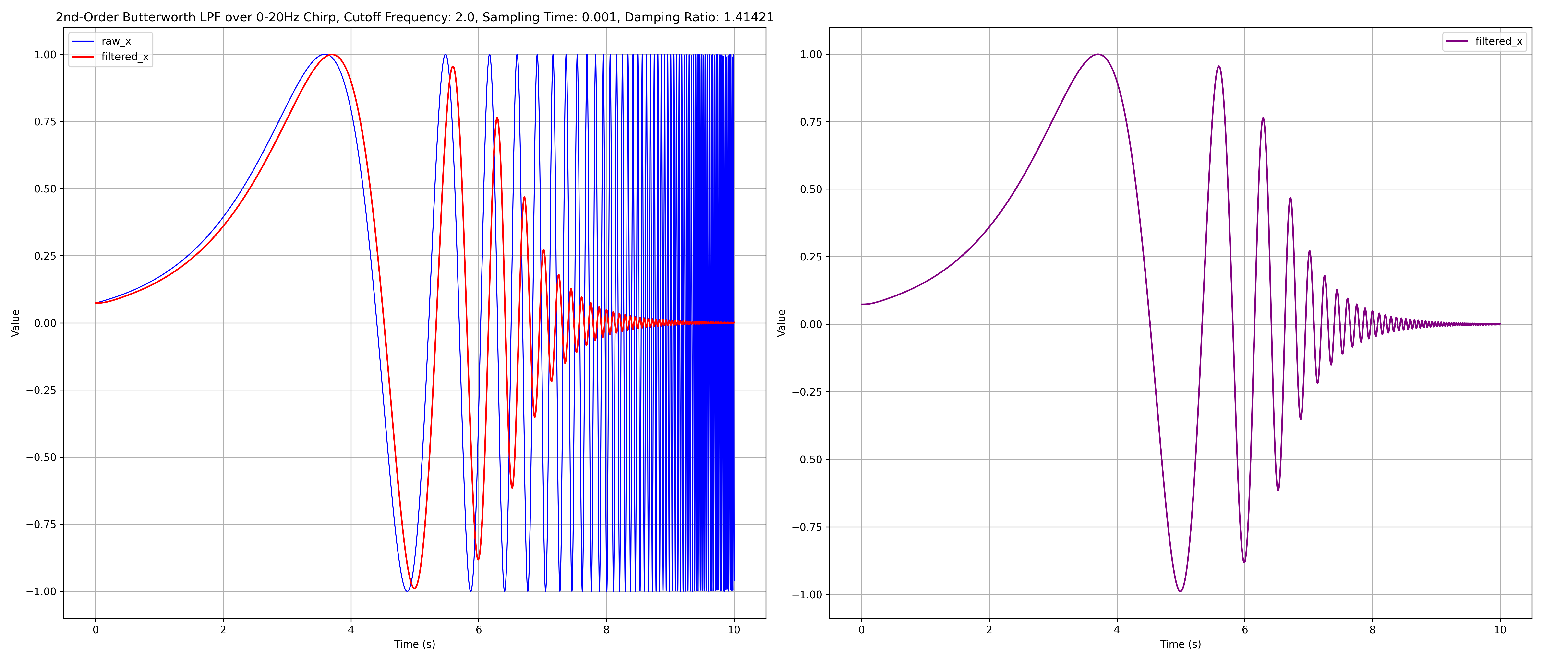
Response of a 2nd-order butterworth filter over Linear and Exponential Chirp signals with $f_0 = 0.01 \text{ Hz}$, $f_1 = 50 \text{ Hz}$, $T=10 \text{ s}$ in time domain.
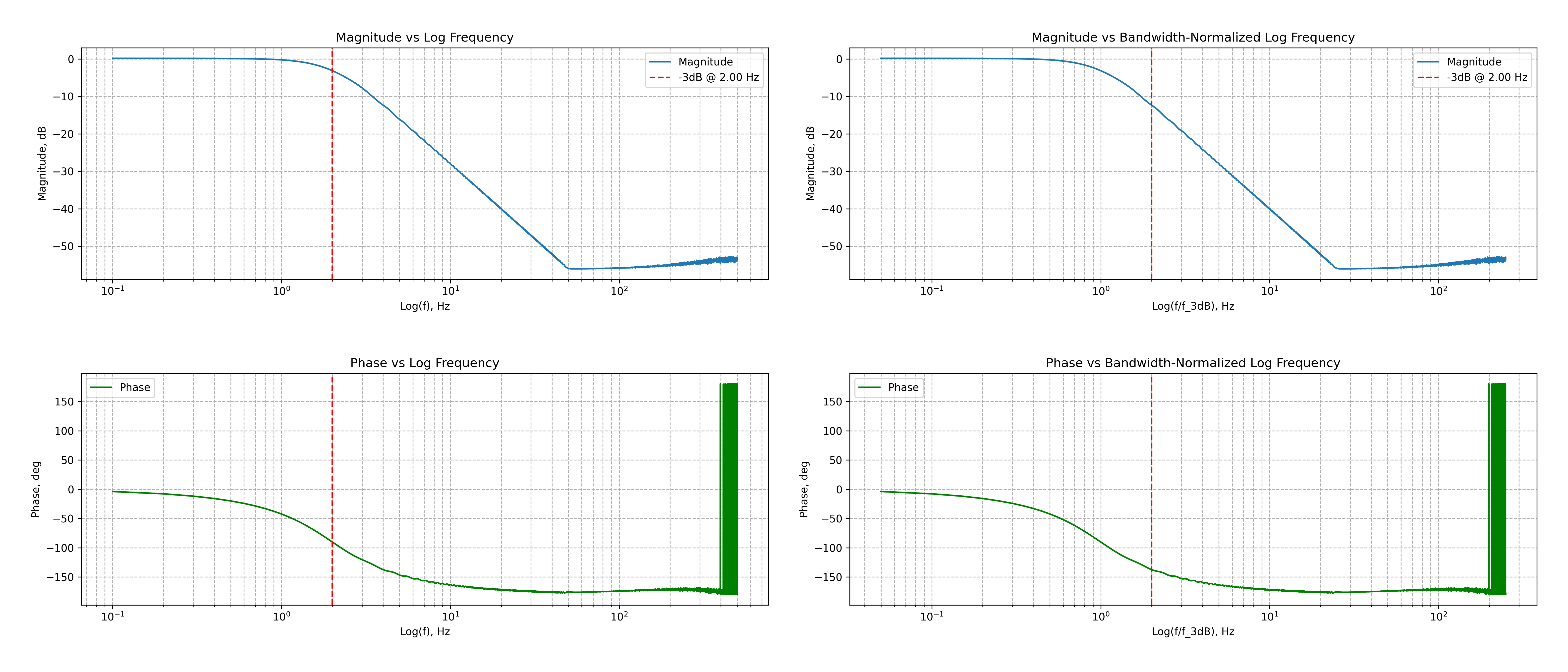
Response of a 2nd-order butterworth filter over a Linear Chirp signals with $f_0 = 0.01 \text{ Hz}$, $f_1 = 50 \text{ Hz}$, $T=10 \text{ s}$ in frequency domain; which corroborates results (-3dB point and slope) shown in Butterworth Filter and Second Order Filters.
Frequency Analysis from Time Domain Data
From chirp response experiments, one gets:
- $ x, y $ - input and output signal time domain sequence, i.e., timestamped points.
One can apply discrete/fast fourier transform (FFT) to get: $$ X = \text{FFT}(x - \bar{x}) $$ $$ Y = \text{FFT}(y - \bar{y}) $$
- $ \bar{x}, \bar{y} $ - input and output signal time domain means, i.e., their DC components,
- $ X, Y $ - input and output signal frequency domain sequence, i.e., complex numbers.
The system transfer function is $$ H(\text{j}\omega) = \frac{Y(\text{j}\omega)}{X(\text{j}\omega)} $$ One can therefore get the frequency response sequence from time response sequence by $$ H = \frac{Y}{X} $$ Then, one can compute its magnitude $A$ and phase $\phi$ by $$ A = 20 \cdot \log_{10}(|H|) $$ $$ \phi = \angle H $$ where computation of $|H|$ and $\angle H$ can be found in Magnitude and Phase of Complex Numbers. Note that only positive frequencies are needed, one can then plot the magnitude over frequency plots, i.e., the bode plots. For reference, see Bode Plot and Bode Plots Explained.