Operational Space Framework, Hybrid Motion-Force Control
Motivation
When a robot has redundant degrees-of-freedom, solving its inverse kinematics can be difficult or less efficient since the solution is not unique. When the control goal is to achieve certain contact force in the Cartesian space, designing controllers based on dynamics models would also be easier than using methods based on robot kinematics. These reasons precipitate the development of Operational Space (a.k.a Task Space) Framework.
This post summarizes some results in 1987@Khatib and describes
- the relationship between joint space and operational space dynamics,
- the most straight forward operational space controller design,
- the physical interpretation of hybrid motion-force control,
- some simplification in practical implementation, and
- some practical issues associated with the operational space approach.
In paper 1987@Khatib , the hybrid motion-force controller is called a unified motion-force controller. However, it's sometimes confusing to discuss "motion-force" (which refers to pose and wrench control goals) and "moment-force" (components of a wrench) together especially when using the $M$ and $F$ notations. So this post refers to the hybrid controller as a pose-wrench controller. In addition, this post sometimes uses force to refer to a generalized force, i.e., a wrench in $\mathbb{R}^6$, it should be clear based on the local context.
Demonstration
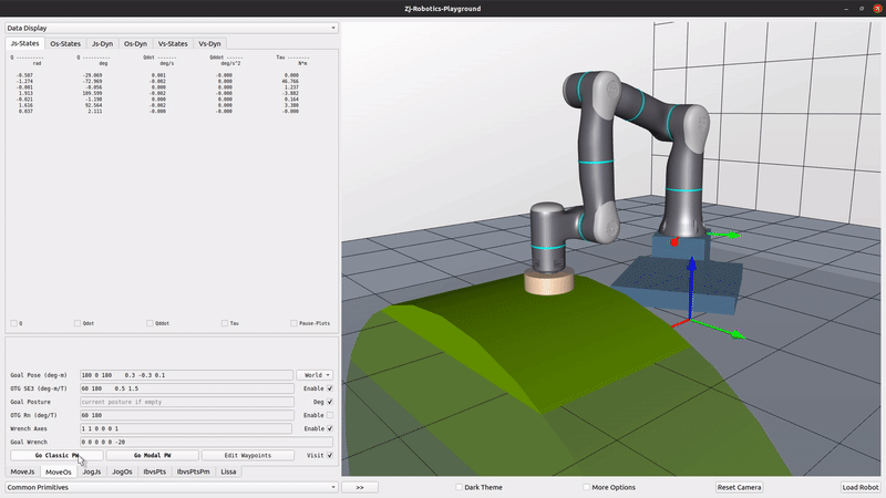
Below demonstrates the optional space (1) motion control and (2) hybrid motion-force control. Notice that the hybrid motion-force control follows the curved surface without knowing its profile due to active force control maintains a desired contact force and moment with the environment.
Nomenclature
In addition to nomenclature used in Fundamentals of Dynamics and Control of Flexible Joint Robots:
- $\{B\}$ - robot base frame
- $\{M\}$ - moment control frame
- $\{F\}$ - force control frame
- $J$ - robot control point Jacobian in $\{B\}$
- $\bar{J}$ - dynamically consistent generalized inverse of $J$
- $\Lambda$ - operational space mass matrix
- $\mu$ - operational space Coriolis force
- $\rho$ - operational space gravity
- $F$ - operational space control generalized force
- $x, \dot{x}, \ddot{x}$ - operational space measured position, velocity, acceleration
- $f$ - operational space measured generalized force
Relationship between Joint and Operational Space Dynamics
A robot's joint space dynamics is given by $$ M\ddot{q} + c + g = \tau $$ note that the external torque is omitted for simplicity of notations. In the operational space, the dynamics has the same form while the terms are different $$ \Lambda \ddot{x} + \mu + \rho = F \label{eq:os-dynamics} $$ The dynamics in the two spaces are related by $$ M\ddot{q} + c + g = \tau \Longleftrightarrow J^T \bigl\{ \Lambda \ddot{x} + \mu + \rho = F \bigl\} \label{eq:dynamics-relationship} $$
As shown in 1987@Khatib , the operational space terms are $$ \Lambda = (J M^{-1} J^T)^{-1} $$ $$ u = \bar{J}^T c - \Lambda \dot{J} \dot{q} $$ $$ \rho = \bar{J}^T g $$ where $$ \bar{J} = M^{-1} J^T \Lambda \label{eq:j-bar} $$ and $$ \bar{J}^T = \Lambda J M^{-1} $$ since $M$ and $\Lambda$ are positive definite symmetric.
The $\bar{J}$ in \eqref{eq:j-bar} is called the dynamically consistent generalized inverse Jacobian in 1987@Khatib . It is also referred to as the inertia-weighted pseudo-inverse of Jacobian in the literature such as in 2008@Nakanishi . Expanding \eqref{eq:j-bar} $$ \bar{J} = \textcolor{red}{M^{-1}} J^T ( J \textcolor{red}{M^{-1}} J^T )^{-1} $$ and comparing it with the canonical definition of the Moore-Penrose pseudo-inverse $$J^+ = J^T(JJ^T)^{-1}$$ for $A\in \mathbb{R}^{m\times n}$ for $n >= m$ as in Ghaoui@2021 , it is not difficult to see why it is also called the inertia-weighted pseudo-inverse of Jacobian. Note that there are other generalized Jacobian inverses that deal with robot redundancy resolution in 2008@Nakanishi and other articles.
The Most Straight Forward Operational Space Controller Design
In order to track an operational space trajectory given by $\bigl\{ x, \dot{x}, \ddot{x} \bigl\}$, a simple impedance plus feedforward controller in the operational space would do $$ F = \Lambda F^* + \mu + \rho \label{eq:operational-space-force} $$ where $$ F^* = -K_p(x - x_d) - K_d(\dot{x} - \dot{x}_d) + \ddot{x}_d \label{eq:motion-impedance-controller} $$
Using the relationship between joint and operational space dynamics given in \eqref{eq:dynamics-relationship}, it is easy to compute the joint torque $$ \tau = J^T F = J^T (\Lambda F^* + \mu + \rho) $$ corresponds to the operational space control force in \eqref{eq:operational-space-force} for operational space trajectory tracking.
Implementation Simplification
In practice, instead of feedforward the Coriolis force and gravity in the operational space, people often compensate for these bias forces in the joint space using $$ \tau = J^T F + c + g $$ with $$ F = \Lambda (F^* - \dot{J} \dot{q}) \label{eq:simplified-operational-space-force} $$ since the joint space gravity and Coriolis force effect are gone in the operational space. Which simplified a lot of unnecessary computation.
Operational Space Unified Pose-Wrench Control
Purpose
To apply operational space unified pose-wrench control is to
- track some desired moment along some directions in $\{M\}$ that takes $R_M$ to rotate to $\{B\}$,
- track some desired force along some directions in $\{F\}$ that takes $R_F$ to rotate to $\{B\}$,
- track some desired orientation and position along some directions complements to the moment and force directions in their correspond frames.
Control Law
One can employ the operational space control law given by \eqref{eq:simplified-operational-space-force}; however, in this case $$ F^* = \Omega F^{*}_{Pose} + \overline{\Omega} F^{*}_{Wrench} \label{eq:unified-control} $$ where the pose control is $$ F^*_{Pose} = -K_p(x - x_d) - K_d(\dot{x} - \dot{x}_d) + \ddot{x}_d \label{eq:motion-control} $$ is the same impedance controller as in \eqref{eq:motion-impedance-controller}; however, the wrench control is $$ F^{*}_{Wrench} = -K_f(f - f_d) - K_d \dot{x} + f_d \label{eq:force-control} $$ with a force error term, a velocity damping term, and a feedforward desired force. This is due to the fact that force derivative is typically difficult to measure and force control often aims at achieving a set of target forces instead of a trajectory with higher order terms.
Physical Interpretation
Motion and force controllers in \eqref{eq:motion-control} and \eqref{eq:force-control} achieve desired motion and force in their own frames $\{M\}$ and $\{F\}$ independently; whereas the controller in \eqref{eq:unified-control} unifies them through the global selection matrix $$ \Omega = \begin{bmatrix} R_M^T \Sigma_M R_M & 0 \\ 0 & R_F^T \Sigma_F R_F \end{bmatrix} \label{eq:global-selection-matrix} $$ with local selection matrices $$ \Sigma_M = \text{diag} \{\sigma_{M_x}, \sigma_{M_y}, \sigma_{M_z} \} $$ $$ \Sigma_F = \text{diag} \{\sigma_{F_x}, \sigma_{F_y}, \sigma_{F_z} \} $$ $$ \sigma \in \{ 0, 1 \} $$ and $ \overline{\Omega} $ complements the selection made by $ \Omega$ via $\overline{\Sigma}_M$ and $\overline{\Sigma}_F$, and $\overline{\sigma}$ that complement $\Sigma_M$ and $\Sigma_F$, and $\sigma$.
The global selection matrix in \eqref{eq:global-selection-matrix} can be interpreted as:
- first rotate the pose control effort from $\{B\}$ to $\{M\}$ and $\{F\}$,
- select axes that are intended to apply orientation and position control locally in $\{M\}$ and $\{F\}$, then
- rotate back the control effort back to $\{B\}$,
Additional Notes
When applying unified pose-wrench control, oftentimes the target control frames are in the robot end-effector frame. In that case, in the global selection matrix \eqref{eq:global-selection-matrix}, there's no need to first rotate the control effort to the local frame, cause there are already in there, i.e.: $$ \Omega = \begin{bmatrix} R_M^T \Sigma_M & 0 \\ 0 & R_F^T \Sigma_F \end{bmatrix} $$
In some other cases, the target control frame could be a user frame $\{U\}$, which is not in the robot base frame. Yet since $J$ is often defined in $\{B\}$, the rotation matrices in the global selection matrix could be different as well, i.e.: $$ \Omega = \begin{bmatrix} \sideset{^B}{_M}{R} \Sigma_M \sideset{^M}{_U}{R} & 0 \\ 0 & \sideset{^B}{_F}{R} \Sigma_F \sideset{^F}{_U}{R} \end{bmatrix} $$ where $\sideset{^M}{_U}{R}$ rotates from $\{U\}$ to $\{M\}$, $\Sigma_M$ does local selection, $\sideset{^B}{_M}{R}$ rotates from $\{M\}$ to $\{B\}$; and so forth for the force control axes.
Practical Issues with the Operational Space Approach
There are some outstanding practical issues with the operational approaches, among them:
- the operational space mass matrix $\Lambda$ only exists outside of singularities, when close to singularity, $\Lambda$ will explode, and
- because of model uncertainties, even when outside of singularities, the $\Lambda$ can still be inaccurate, which will negatively affect control performance, especially the inaccurately estimation of the off-diagonal terms in $\Lambda$, will cause very undesirable behaviors.
Task-Consistent Recursive Nullspace Control
In addition to allowing direct design of controller in the task space, another advantage of the operational space approach is that the formulation allows one to handle redundant robot in a fairly straight forward manner. The dynamically consistent generalized inverse of Jacobian leads to dynamically consistent nullspace. Which can be formulated recursively to deal with multiple tasks with strict priorities. Details on that will be discussed in another post.
Comparison of Different Hybrid Motion-Force Control Formulations
Besides methods proposed in 1987@Khatib , there are other ways to achieve pose-wrench control with even better performance.
For example, the Hybrid Motion-Force Controller in Sec. 11.6.2 in 2017@Lynch is able to control motion and force at the same time and places the force control with a strictly higher priority. Which is mathematically equivalent to creating a force control task and motion control task and stack them using the prioritized multitask controller in 2005@Sentis .
The Pfaffian constraint matrix $A$ in 2017@Lynch and subsequently involves in the computation of the projection matrix $P$, can be interpreted as a matrix that selects rows from a column vector. For example, if the Pfaffian constraints prohibit motion in the $\theta_z$ and $y$ direction in $$ \mathcal{V} = \begin{bmatrix} \dot{\theta}_x & \dot{\theta}_y & \dot{\theta}_z & \dot{x} & \dot{y} & \dot{z} \end{bmatrix}^T $$ then an $A$ matrix in the form of $$ A = \begin{bmatrix} 0 & 0 & 1 & 0 & 0 & 0 \\ 0 & 0 & 0 & 0 & 1 & 0 \end{bmatrix} $$ will result in $$ A\mathcal{V} = \begin{bmatrix} \dot{\theta}_z \\ \dot{y} \end{bmatrix} = \mathbf{0} $$ and $$ A\dot{\mathcal{V}} + \dot{A}\mathcal{V} = \begin{bmatrix} \ddot{\theta}_z \\ \ddot{y} \end{bmatrix} + \mathbf{0} = \mathbf{0} $$ hence captures the Pfaffian constraint. The rest of the formulation can easily follow Sec. 11.6.2 in 2017@Lynch .