Constrained Optimization, Lagrange Multiplier
Motivation
Optimization is used everywhere in engineering. In robotics, formulating problems as optimization problems has shown to be more general than solving them in a pure analytical fashion. In particular, it is easier to get solutions via optimization that minimize costs and consider constraints other than dynamics and kinematics, which are typically difficult to handle using pure analytical approach.
This post summarizes some core concepts in Khan@ConOpt and Bazett@LagMul to provide some physical intuition behind the optimization approach. It focuses on optimization problems with one constraint for simplicity. Optimization problems with multiple constraints will be discussed in a separate post.
Some matrix and vector calculus identities are used in the derivation of, for example, the partial derivative of a quadratic matrix term. These identities can be found in Wikipedia@MatCal , Wikipedia@VecCal , and Wikipedia@Grad .
Nomenclature
In addition to notations used in Operational Space Framework, Hybrid Motion-Force Control, the following nomenclature is used.
- $ \lambda $ - Lagrange multiplier, $ \lambda \in \mathbb{R}$ in the single constraint case
- $ \mathbf{x} $ - Optimization variable, $ \mathbf{x} \in \mathbb{R}^n $
- $ f(\mathbf{x}) $ - objective function, $ f: \mathbb{R}^n \mapsto \mathbb{R} $, sometimes written as $f$ for simplicity
- $ g(\mathbf{x}) $ - constraint function, $ g: \mathbb{R}^n \mapsto 0 $, sometimes written as $g$ for simplicity
- $ \mathcal{L}(\mathbf{x}, \lambda) $ - Lagrangian $ \mathcal{L}: \mathbb{R}^{n+1} \mapsto \mathbb{R} $, sometimes written as $\mathcal{L}$ for simplicity
- $ \nabla_{\mathbf{x}} \mathcal{X}(\mathbf{x}) $ - function gradient, $ \nabla_{\mathbf{x}} \mathcal{X}(\mathbf{x}) = \frac{\partial \mathcal{X}(\mathbf{x})}{\partial \mathbf{x}} = \begin{bmatrix} \frac{\partial \mathcal{X}}{\partial x_1}, \frac{\partial \mathcal{X}}{\partial x_2}, \cdots, \frac{\partial \mathcal{X}}{\partial x_n} \end{bmatrix}^T $, sometimes written as $\nabla \mathcal{X}(\mathbf{x})$, $\nabla \mathcal{X}$, or $\frac{\partial \mathcal{X}}{\partial \mathbf{x}}$ for simplicity
Problem Formulation and Physical Meaning
A single constrained optimization problem can be formulated as follows. $$ \begin{align} \underset{\mathbf{x}}{\text{maximize}} \hspace{0.2in} &f(\mathbf{x}) \label{eq:objective} \\ \text{subject to} \hspace{0.2in} &g(\mathbf{x}) = 0 \label{eq:cost} \end{align} $$ Mathematician Joseph-Louis Lagrange shows that the optimal solution of such a problem can be found by solving $$ \nabla f(\mathbf{x}) = \lambda \nabla g(\mathbf{x}) \label{eq:solution} $$
The physical meaning of such a solution can be explained in the $\mathbf{x} \in \mathbb{R}^2$ case as follows.
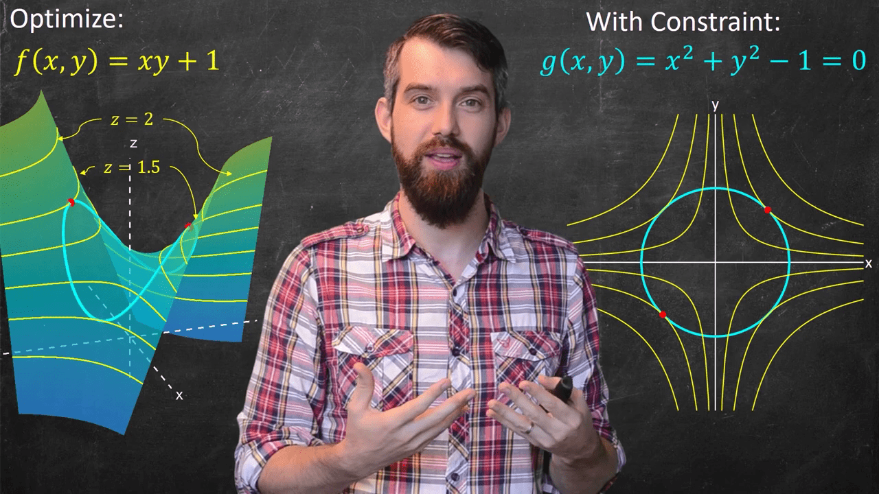
- $ f(\mathbf{x}) $ is a 3D contour that for each $\mathbf{x}$ in XY-plane, there is an associated Z-value to it,
- $ g(\mathbf{x}) $ is a curve that lies in the XY-plane,
- the optimization problem is to choose a point from $ g(\mathbf{x}) $ in the XY-plane, that optimizes the output Z-value of $ f(\mathbf{x}) $,
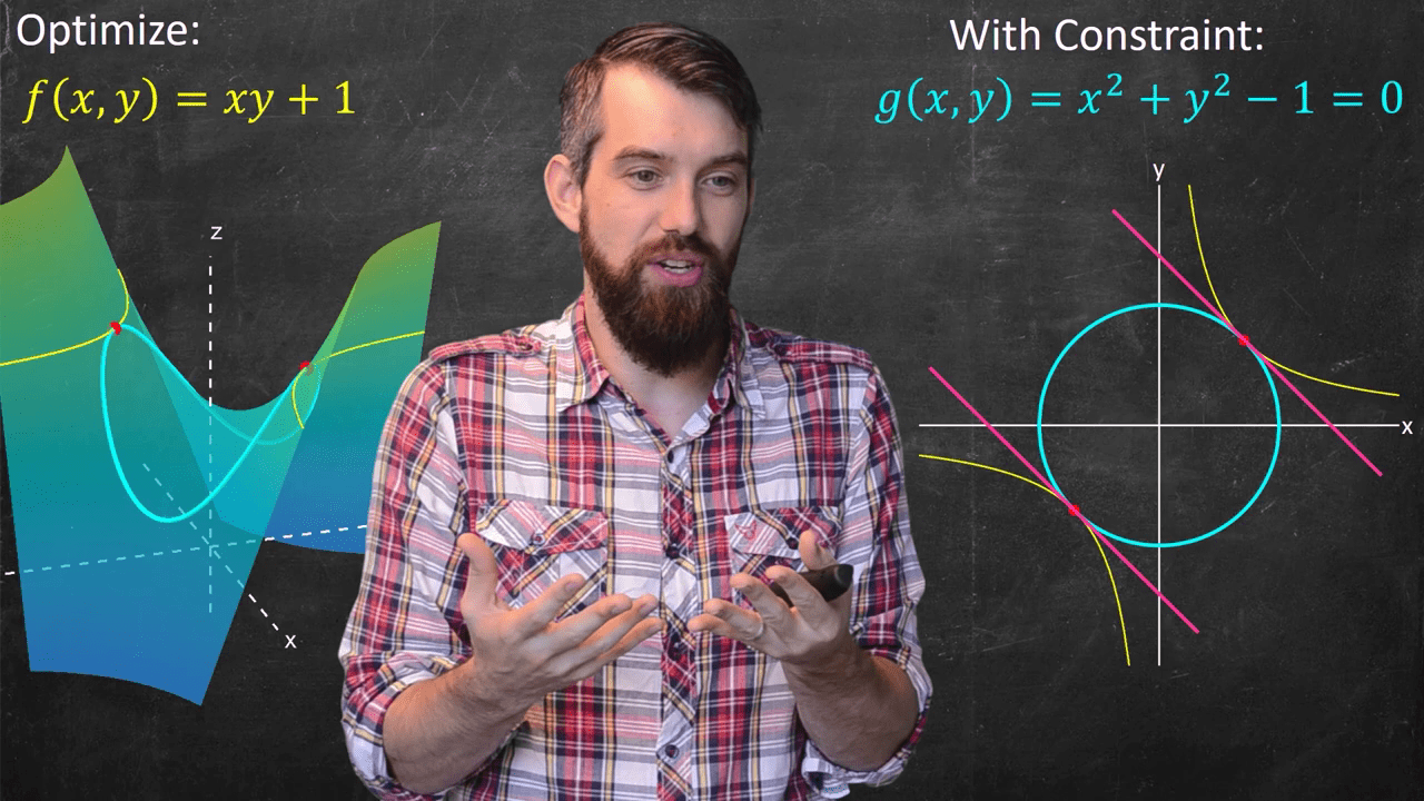
- the Lagrange solution says that such a point must be at where the gradient of $f(\mathbf{x})$ and $g(\mathbf{x})$ are parallel to each other.
Visual Interpretation
Visually, the following figures from Bazett@LagMul clearly illustrate the concept in the $\mathbf{x} \in \mathbb{R}^2$ case. That is, the optimal solutions can be found from:
- Fig. 1: level sets in $f(\mathbf{x})$ that barely touch the constraint curve,
- Fig. 2: "barely touching" condition can be geometrically captured by the tangential condition of level sets in $f(\mathbf{x})$ and curve $g(\mathbf{x})$,
- Fig. 3: curves tangential to each other can be further captured by gradients parallel to each other.

The concept is difficult to visualize beyond $\mathbf{x} \in \mathbb{R}^2$. However, the mathematics can generalize to $\mathbf{x} \in \mathbb{R}^n$ and the principles still hold.
The Lagrangian Formulation
Another way to formulate the optimization problem in \eqref{eq:objective}, \eqref{eq:cost}, and their solution in \eqref{eq:solution} is to write a Lagrangian, $$ \mathcal{L}(\mathbf{x}, \lambda) = f(\mathbf{x}) - \lambda g(\mathbf{x}) \label{eq:lagrangian} $$ and solve for $$ \nabla_{\mathbf{x}, \lambda} \, \mathcal{L}(\mathbf{x}, \lambda) = \mathbf{0} \label{eq:lagrangian-solution} $$ that expands to $$ \begin{align} \frac{\partial \mathcal{L}}{\partial \mathbf{x}} &= \frac{\partial f(\mathbf{x})}{\partial \mathbf{x}} - \lambda \frac{\partial g(\mathbf{x})}{\partial \mathbf{x}} = \mathbf{0} \\ \frac{\partial \mathcal{L}}{\partial \lambda} &= g(\mathbf{x}) = \mathbf{0} \end{align} $$ which is exactly the same as the original problem and the optimal solution, packed in a more elegant way. Refer to Khan@ConOpt for a more complete explanation and the meaning of the Lagrange Multiplier value in the optimal solution.
In addition, note that \eqref{eq:lagrangian} is a new function, and \eqref{eq:lagrangian-solution} is its gradient equal to zero, corresponding to the optimal solution. So, the Lagrangian formulation actually converts the original constrained optimization problem into an unconstrained optimization problem, which often referred to as the dual of the original/primal problem. Details of the primal-dual problems will be discussed in a separate post. The meaning of the Lagrange Multipliers value in the optimal solution becomes more obvious in the primal-dual min-max problems setting.
Additional Notes
Sometimes the constraint is written as $$ g(\mathbf{x}) = c $$ for $c\in \mathbb{R}$, which doesn't change the problem since one can convert it back to the standard form by writing $$ \mathsf{g}(\mathbf{x}) = g(\mathbf{x}) - c = 0$$ The same goes for the object function, minimizing a function $f(x)$ can be written as maximizing $-f(x)$.
Whether the optimal solution given by \eqref{eq:lagrangian-solution} is maximum or minimum may be determined by:
- checking the definiteness of the bordered Hessian matrix of $\mathcal{L}(\mathbf{x}, \lambda)$ evaluated at the optimal point $(\mathbf{x}^*, \lambda^*$),
- comparing among all optimal solutions.
But more often than not, it's not a concern since the optimization package will set up the problem in a standard form and either minimize or maximize the objective based on some configuration. The important thing is to either (1) understand the physical meaning and formulate problems as standard optimization problems for numerical packages to solve, or (2) derive the analytical solution for some simple problems.