Image-Based Visual Servo Control
Motivation
Tracking a moving object based on vision feedback is a common task in robotics. One approach to realize such object tracking is called image-based visual servo (IBVS) control. In IBVS, the vision system detects a set of $\mathbb{R}^2$ features (each associated with a scalar depth) fixed on the object; based on some desired $\mathbb{R}^2$ targets in the image space, IBVS scheme generates robot motion that reduces the error between detected features and their target to zero in the image space to realize Cartesian space object tracking.
IBVS is known for its insensitivity to camera extrinsic parameter (install and calibration) uncertainties. Since the control law mostly relies on camera intrinsic parameters (optical structure and projection), which are often very accurate because of their manufacturing process. As a result, IBVS is often used in high precision object alignment and tracking control.
This post summarizes some results in 1996@Hutchson , 2006@Chaumette , 2007@Chaumette , and compares IBVS with position-based visual servo (PBVS). This post uses IBVS with point features as an example for simplicity to explain IBVS theory and its physics. For an introduction to camera model, calibration, intrinsic and extrinsic parameters, see MathWorks@CamCali .
Demonstration
Below shows the kinematics relationship between feature and camera velocity through interaction matrix (or image Jacobian) and IBVS aligning four detected points features to their desired targets in the image space in simulation.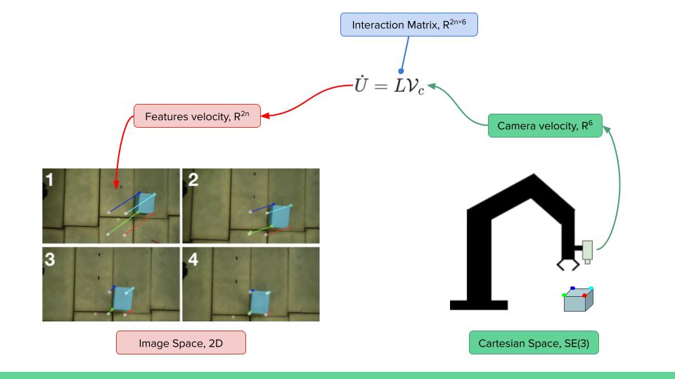

Nomenclature
- $c_x, c_y$ - camera optical center coordinates, $c_x, c_y, \in \mathbb{R}^+$ in pixels
- $f_x, f_y$ - camera focal length, $f_x, f_y, \in \mathbb{R}^+$ in pixels
- $u, \nu$ - feature coordinate in the image space, $u, \nu, \in \mathbb{R}^+$ in pixels
- $x, y$ - normalized point feature coordinates, $x, y \in [-1,1]$
- $Z$ - feature depth, $Z\in\mathbb{R}^+$ in meters along the camera sensing direction $z$-axis
- $x^*, y^*, Z^*$ - desired feature coordinates and depth
- $\mathcal{V}_c$ - camera velocity in its body frame, $\mathcal{V}_c \in \mathbb{R}^6$
- $L$ - feature image Jacobian, also referred to as interaction matrix, for a single feature $L\in\mathbb{R}^{2\times6}$, for a stack of $n$ features $L\in\mathbb{R}^{2n\times6}$
- $\dot{U}$ - feature velocity in its normalized coordinates with $\dot{U} = \begin{bmatrix} \dot{x} & \dot{y} \end{bmatrix}^T$, for a single feature $\dot{U} \in \mathbb{R}^2$, for a stack of $n$ features $\dot{U} \in \mathbb{R}^{2n}$
Feature and Camera Velocity Kinematics
The key to IBVS is to establish the relationship between camera motion and the motion of features appear in the camera's image space. Such relationship can be established through their velocity kinematics via feature interaction matrices.
Take a point feature for example, such a relationship is governed by the point feature interaction matrix. It maps camera velocity $\mathcal{V}_c$ in its body frame, to feature velocity $\dot{U}$ in the normalized camera image space. $$ \dot{U} = L \mathcal{V}_c = \begin{bmatrix} \begin{array}{c:c} L_{\omega} & L_v \end{array} \end{bmatrix} \, \mathcal{V}_c \label{eq:ibvs-kinematics} $$ which expands to $$ \begin{bmatrix} \dot{x} \\ \dot{y} \end{bmatrix} = \begin{bmatrix} \begin{array}{ccc:ccc} xy & -(1+x^2) & y & -\frac{1}{Z} & 0 & \frac{x}{Z} \\ 1+y^2 & -xy & -x & 0 & -\frac{1}{Z} & \frac{y}{Z} \end{array} \end{bmatrix} \begin{bmatrix} \omega_c \\ v_c \end{bmatrix} \label{eq:interaction} $$ where $L_{\omega}, L_v \in \mathbb{R}^{3\times2}$ are the angular and linear partitions of the image Jacobian, $\omega_c, v_c \in \mathbb{R}^3$ are the camera's angular and linear velocity.
To convert from original feature coordinates $(u, \nu)$ directly measured by the camera in pixels, to the normalized coordinates used in \eqref{eq:ibvs-kinematics}, the following relationship applies $$ x = \frac{u - c_x}{f_x} $$ $$ y = \frac{\nu - c_y}{f_y} $$
In order to fully control the camera motion (6-DOF), there has to be at least 3 features ( $3\times2$-DOF), to establish a fully actuated kinematics mapping. But it's common practice to at least provide 4 features for fully control the camera's motion. When there are $ n $ features in the image, the image Jacobian can be composed by stacking of the individual image point Jacobians, and the governing equation becomes $$ \begin{bmatrix} \dot{x}_1 \\ \dot{y}_1 \\ \dot{x}_2 \\ \dot{y}_2 \\ \vdots \\ \dot{x}_n \\ \dot{y}_n \end{bmatrix} = \begin{bmatrix} L_{\omega,1} && L_{v,1} \\ L_{\omega,2} && L_{v,2} \\ \vdots && \vdots \\ L_{\omega,n} && L_{v,n} \end{bmatrix}_{2n \times 6} \begin{bmatrix} \omega_c \\ v_c \end{bmatrix} $$
Computing Camera Velocity in $\mathbb{R}^6$
Taking one feature point as an example for simplicity, the camera body velocity is given by $$ \mathcal{V}_c = L^{\dagger} \begin{bmatrix} \dot{x} \\ \dot{y} \end{bmatrix} $$ To get the normalized features to converge to some desired targets $x_d, y_d$, the simplest control law is to design the camera velocity to be $$ \mathcal{V}_c = L^{\dagger} \cdot k_p \begin{bmatrix} -(x - x_d) \\ -(y - y_d) \end{bmatrix} $$ which renders the feature space error dynamics as $$ \begin{bmatrix} \dot{x} \\ \dot{y} \end{bmatrix} = L L^{\dagger} \cdot k_p \begin{bmatrix} -(x - x_d) \\ -(y - y_d) \end{bmatrix} $$ which approaches to zero exponentially fast under nominal conditions with \( k_p \in \mathbb{R}^+ \).
Computing Camera Pose in $SE(3)$
When camera body velocity is known, one can get the camera pose increment \( \Delta X_c \in SE(3) \) in a small amount of time \( \Delta t \) by $$ \Delta X_c = \begin{bmatrix} \Delta R & \Delta p \\ 0 & 1 \end{bmatrix} = \begin{bmatrix} Rot(\frac{\omega_c}{||\omega_c||}, ||\omega_c|| \Delta t) & v_c \Delta t \\ 0 & 1 \end{bmatrix} $$ Since the camera pose increment \( \Delta X_c \in SE(3) \) is induced by the camera body velocity, so \( \Delta X_c \) is a transformation w.r.t. the camera's body frame.
Thus, if one knows the camera's current pose in world \( X^k_c \in SE(3) \), one can get the camera's new pose in world \( X^{k+1}_c \in SE(3) \) via $$ X_c^{k+1} = X_c^{k} \cdot \Delta X_c $$ with a right multiplication of the incremental pose, since the transformation is performed w.r.t. the camera's body frame. In contrast to left multiplication, indicating the transformation performed w.r.t. the fixed world frame.
Computing Robot End-Effector Pose in $SE(3)$
Since both the camera velocity and pose is known for tracking a set of features, there are two ways to control the robot end-effector motion.
Assuming the camera is fixed w.r.t. the end-effector, which is referred to a eye-in-hand configuration, then one can convert the camera's pose to the end-effector's pose for robot control using method such as described in Operational Space Framework, Hybrid Motion-Force Control.
Or, one can compute the desired end-effector velocity from the desired camera velocity through a plucker transformation, then compute the new end-effector pose using the method mentioned in the previous section.
Practical Implementation
Estimating depth of a feature is often difficult or difficult to yield high quality results due to noise. In practice, people often use desired depth to compose the interaction matrix. That is, instead of using all estimated $x, y, Z$ in \eqref{eq:interaction}, an alternative interaction matrix in the form of $$ L^* = \begin{bmatrix} \begin{array}{ccc:ccc} xy & -(1+x^2) & y & -\frac{1}{Z^*} & 0 & \frac{x}{Z^*} \\ 1+y^2 & -xy & -x & 0 & -\frac{1}{Z^*} & \frac{y}{Z^*} \end{array} \end{bmatrix} \label{eq:interaction-desire} $$ is often employed to achieve IBVS, where $Z^*$ is the desired feature depth.
Such an alternative often yields better control performance and results in practice. And one can notice from \eqref{eq:interaction-desire}, that this alternation only affects the camera's linear motion since the angular motion partition of the interaction matrix does not involve feature depth.
Scheme Comparison
IBVS and PBVS both have their pros and cons, which one is a better choice for an application depends on many factors. Below is a basic comparison between the two. PBVS scheme will be discussed in a separate post.| Control Scheme | IBVS | PBVS |
|---|---|---|
| Vision system input | Feature x, y position in camera space \( \in \mathbb{R}^2 \) | Object pose in Cartesian \( SE(3) \) space |
| Camera calibration | Insensitive
|
Sensitive
|
| Precision | High
|
Low
|
| Algorithm complexity |
High, 6 steps:
|
Low, 1 step:
|
Additional Notes
This post describes the basics of IBVS, there are more aspects to consider, some of them are listed below.
- Image Jacobian singularity handling
- Velocity integral control handling
- Second-order control
- Partitioned IBVS
- Cartesian velocity constraints
- Feature depth observer
- Vision-impedance control
- Line features, circle features, image moments
- Feature velocity Kalman filtering
- Hybrid IBVS-PBVS control
- Eye-in-hand and eye-to-hand
- Homography and multi-camera IBVS
- Pattern matching with IBVS
- Image space boundary potential field